
Last updated April 2026 — refreshed for current algorithm analysis, modern use cases, and 2026 interview relevance.
Searching algorithms sit at the heart of nearly every software system: databases, file systems, vector search engines, and your git bisect debugging workflow all rely on the same fundamental ideas. This guide covers every major classical search algorithm with precise complexity numbers, working code in Java and Python, a comparison table, a decision framework, and a section on where these ideas show up in modern production systems — including vector databases and AI search pipelines.
What changed since 2023
- Vector / ANN search is now mainstream. Approximate Nearest Neighbor algorithms (HNSW, IVF-PQ) implemented in Milvus, Pinecone, pgvector, and Supabase are the "search" layer for every RAG-based AI application as of 2025–2026. Classic algorithms still underpin them internally.
- git bisect is a canonical binary search example. As of Git 2.44+ the algorithm is explicitly documented as binary search; it has become the go-to real-world illustration for engineering interviews.
- Python 3.12
bisectmodule is C-accelerated by default. The pure-Python fallback was removed in CPython 3.12;bisect.bisect_left/bisect_rightare now always O(log n) with a tight constant factor. - B-tree and B+ tree remain the default for persistent storage. PostgreSQL 16, MySQL 8.4, and SQLite 3.45 all ship B+ tree as the default index — binary search on each node, O(log n) disk reads.
- Hash tables beat binary search for point lookups when data is volatile. For large mutable key-value stores (Redis 7.x, Memcached) amortized O(1) hash lookup is preferred over sorted-array binary search.
What is a Search Algorithm?
A search algorithm is a procedure that retrieves an element from a data structure given a key (search target). All search algorithms have two possible outcomes: found (returns index or reference) or not found (returns -1 or null). Algorithms are classified primarily by two properties:
- Sequential search — traverse elements one by one (Linear Search). No precondition on ordering.
- Interval search — exploit sorted order to eliminate large portions of the search space in each step (Binary Search, Jump Search, Fibonacci Search, Interpolation Search, Exponential Search).
A third modern class — hashing and approximate search — trades exact results or memory for dramatically faster lookups and is covered in the decision framework at the end of this post.
TL;DR: Algorithm Comparison Table
| Algorithm | Best case | Average case | Worst case | Space | Requires sorted data? | Best for |
|---|---|---|---|---|---|---|
| Linear Search | O(1) | O(n) | O(n) | O(1) | No | Small / unsorted lists |
| Binary Search | O(1) | O(log n) | O(log n) | O(1) iterative | Yes | Large sorted arrays |
| Jump Search | O(1) | O(√n) | O(√n) | O(1) | Yes | Sorted arrays, backward jump is expensive |
| Interpolation Search | O(1) | O(log log n) | O(n) | O(1) | Yes + uniform | Uniformly distributed sorted data |
| Exponential Search | O(1) | O(log n) | O(log n) | O(1) iterative | Yes | Unbounded / infinite arrays |
| Fibonacci Search | O(1) | O(log n) | O(log n) | O(1) | Yes | No division operator available (embedded) |
| Hash Table Lookup | O(1) | O(1) | O(n) | O(n) | No | Point lookups, key-value stores |
| HNSW (ANN) | O(log n) | O(log n) | O(n) | O(n) | No | High-dimensional vector similarity |
Types of Searching Algorithms
- Linear Search
- Binary Search
- Jump Search
- Interpolation Search
- Exponential Search
- Sublist Search
- Fibonacci Search
- The Ubiquitous Binary Search (advanced patterns)

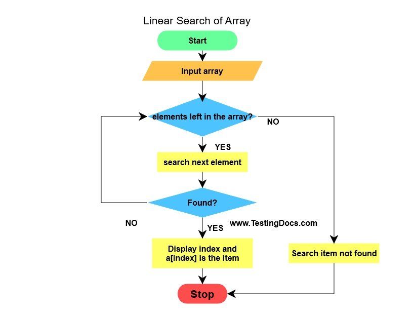
Linear Search
A linear search (also called sequential search) checks each element of the list one by one from the start until the target is found or the list is exhausted. It makes no assumption about the ordering of data.
- Time complexity: O(n) worst and average case; O(1) best case (target at index 0).
- Space complexity: O(1).
- When to use: Small lists (<20 items), unsorted data where sorting overhead is not worth it, single searches on dynamic data.
Java
// Returns index of x in arr[], or -1 if not present
public static int linearSearch(int[] arr, int x) {
    for (int i = 0; i < arr.length; i++) {
        if (arr[i] == x) return i;
    }
    return -1;
}
Python
def linear_search(arr, x):
    for i, val in enumerate(arr):
        if val == x:
            return i
    return -1
Pitfall: Using linear search on a sorted list is always a mistake if you plan to search it more than once. Sort once, then use binary search for every subsequent lookup — the break-even is roughly 7–10 searches on lists of 1,000+ elements.
Binary Search
Binary search is the standard algorithm for sorted arrays. It uses divide and conquer: compare the target to the middle element, then eliminate half the remaining search space. Also known as half-interval search or logarithmic search.
- Time complexity: O(log n) worst and average; O(1) best (target at midpoint).
- Space complexity: O(1) iterative; O(log n) recursive (call stack).
- Precondition: Array must be sorted.
For a sorted array of 1,000,000 elements, binary search takes at most 20 comparisons (log₂(1,000,000) ≈ 19.9). Linear search would take up to 1,000,000 comparisons in the worst case.
Java — iterative (preferred for interviews and production)
// Returns index of x in arr[l..r], or -1 if not present
public static int binarySearch(int[] arr, int l, int r, int x) {
    while (l <= r) {
        int mid = l + (r - l) / 2;  // avoids integer overflow vs (l+r)/2
        if (arr[mid] == x) return mid;
        if (arr[mid] < x)  l = mid + 1;
        else                r = mid - 1;
    }
    return -1;
}
Python — using the standard library
import bisect

def binary_search(arr, x):
    """Returns index of x in sorted arr, or -1."""
    idx = bisect.bisect_left(arr, x)
    if idx < len(arr) and arr[idx] == x:
        return idx
    return -1
In Python 3.12+, bisect.bisect_left is always the C-accelerated version — use the standard library rather than reimplementing.
Real-world example: git bisect
When you run git bisect start, Git performs binary search over your commit history to find the first bad commit. With 1,000 commits to test, git bisect isolates the culprit in at most 10 steps — the same logarithmic efficiency as binary search on a sorted array.
git bisect start
git bisect bad HEAD          # current commit is broken
git bisect good v2.3.0       # this tag was known-good
# Git checks out the midpoint commit; you test, then:
git bisect good              # or: git bisect bad
# Repeat ~10 times for 1000 commits
git bisect reset             # restore HEAD
Binary search in standard libraries
- Java:
Arrays.binarySearch(arr, key)— O(log n), returns negative insertion point if not found. - Python:
bisect.bisect_left,bisect.bisect_right— O(log n), C-accelerated in CPython 3.12+. - C++:
std::lower_bound,std::upper_bound,std::binary_searchin<algorithm>. - JavaScript: No built-in; use a library or implement manually.
Jump Search
Jump search divides the sorted array into blocks of size √n and jumps forward one block at a time until the block that might contain the target is found, then performs a linear search within that block.
- Time complexity: O(√n). Optimal block size is √n, which minimizes total comparisons to 2√n in the worst case.
- Space complexity: O(1).
- When to use: Sorted arrays where backward jumps (as in binary search) are expensive — e.g., sequential-access media or certain network-stored data structures.
Java
public static int jumpSearch(int[] arr, int x) {
    int n = arr.length;
    int step = (int) Math.sqrt(n);
    int prev = 0;

    while (arr[Math.min(step, n) - 1] < x) {
        prev = step;
        step += (int) Math.sqrt(n);
        if (prev >= n) return -1;
    }
    while (arr[prev] < x) {
        prev++;
        if (prev == Math.min(step, n)) return -1;
    }
    return (arr[prev] == x) ? prev : -1;
}
Python
import math

def jump_search(arr, x):
    n = len(arr)
    step = int(math.sqrt(n))
    prev = 0

    while arr[min(step, n) - 1] < x:
        prev = step
        step += int(math.sqrt(n))
        if prev >= n:
            return -1

    while arr[prev] < x:
        prev += 1
        if prev == min(step, n):
            return -1

    return prev if arr[prev] == x else -1
Interpolation Search
Interpolation search improves on binary search for uniformly distributed sorted data by probing at an estimated position rather than always the midpoint. The probe formula is:
pos = lo + ((hi - lo) / (arr[hi] - arr[lo])) * (x - arr[lo])
- Time complexity: O(log log n) average for uniform distributions; O(n) worst case when data is highly skewed.
- Space complexity: O(1).
- When to use: Large, sorted arrays with roughly uniform numeric values — phone directories sorted by number, sorted IP address tables, scientific datasets with evenly spaced measurements.
- When NOT to use: Non-uniform or categorical data; the worst-case degradation to O(n) can be worse than binary search in practice.
Java
public static int interpolationSearch(int[] arr, int lo, int hi, int x) {
    while (lo <= hi && x >= arr[lo] && x <= arr[hi]) {
        if (lo == hi) {
            return (arr[lo] == x) ? lo : -1;
        }
        int pos = lo + ((hi - lo) / (arr[hi] - arr[lo])) * (x - arr[lo]);
        if (arr[pos] == x) return pos;
        if (arr[pos] < x)  lo = pos + 1;
        else                hi = pos - 1;
    }
    return -1;
}
Python
def interpolation_search(arr, lo, hi, x):
    while lo <= hi and arr[lo] <= x <= arr[hi]:
        if lo == hi:
            return lo if arr[lo] == x else -1
        pos = lo + ((hi - lo) * (x - arr[lo])) // (arr[hi] - arr[lo])
        if arr[pos] == x:
            return pos
        if arr[pos] < x:
            lo = pos + 1
        else:
            hi = pos - 1
    return -1
Exponential Search
Exponential search works in two phases: it first finds a range [1, 2, 4, 8, ...] that contains the target, then performs binary search within that range. It is particularly well-suited for unbounded or infinite sorted lists.
- Time complexity: O(log n).
- Space complexity: O(1) iterative.
- When to use: Sorted lists where the size is unknown at runtime, or where the target element is likely near the beginning of the array.
Java
public static int exponentialSearch(int[] arr, int n, int x) {
    if (arr[0] == x) return 0;
    int i = 1;
    while (i < n && arr[i] <= x) i *= 2;
    return binarySearch(arr, i / 2, Math.min(i, n - 1), x);
}
Python
import bisect

def exponential_search(arr, x):
    if arr[0] == x:
        return 0
    i = 1
    while i < len(arr) and arr[i] <= x:
        i *= 2
    sub = arr[i // 2: min(i, len(arr))]
    idx = bisect.bisect_left(sub, x)
    if idx < len(sub) and sub[idx] == x:
        return i // 2 + idx
    return -1
Sublist Search
Sublist search checks whether one linked list appears as a contiguous subsequence within another linked list. It is not commonly used in production but appears in interviews as a test of pointer manipulation and pattern-matching intuition.
Algorithm:
- Take the first node of the second (larger) list.
- Try to match the first list starting from this node.
- If all nodes match, return true.
- Otherwise, advance the second list by one node and repeat.
- If the second list is exhausted without a match, return false.
Time complexity: O(m × n) where m is the length of the sublist and n is the length of the main list. Space complexity: O(1).
Fibonacci Search
Fibonacci search uses Fibonacci numbers to divide the array into unequal parts (approximately 1/3 and 2/3), instead of equal halves. It avoids the division operator, making it suitable for environments where division is expensive (certain embedded CPUs).
- Time complexity: O(log n).
- Space complexity: O(1).
- Advantage over binary search: Examines elements closer to the current position, which can be cache-friendly for very large arrays that don't fit in CPU cache.
Key insight: F(n-2) ≈ (1/3) × F(n) and F(n-1) ≈ (2/3) × F(n), so the algorithm always eliminates roughly one-third of the remaining search space per step.
Java
public static int fibonacciSearch(int[] arr, int x) {
    int n = arr.length;
    int fib2 = 0, fib1 = 1, fibM = fib2 + fib1;

    while (fibM < n) {
        fib2 = fib1;
        fib1 = fibM;
        fibM = fib2 + fib1;
    }

    int offset = -1;
    while (fibM > 1) {
        int i = Math.min(offset + fib2, n - 1);
        if (arr[i] < x) {
            fibM = fib1; fib1 = fib2; fib2 = fibM - fib1;
            offset = i;
        } else if (arr[i] > x) {
            fibM = fib2; fib1 -= fib2; fib2 = fibM - fib1;
        } else {
            return i;
        }
    }
    if (fib1 == 1 && arr[offset + 1] == x) return offset + 1;
    return -1;
}

The Ubiquitous Binary Search — Advanced Patterns
Standard binary search finds an exact match. The real interview power of binary search comes from its variants that find boundary conditions on sorted data. Understanding these patterns solves a large family of LeetCode hard problems.
Pattern 1: Find floor value (largest element ≤ key)
Use a single-comparison loop: advance the left pointer when arr[mid] <= key, advance the right pointer otherwise. When the loop exits, arr[l] is the floor.
// Invariant: arr[l] <= key < arr[r]
// Input: arr[l..r-1], precondition arr[l] <= key
int floor(int[] arr, int l, int r, int key) {
    while (r - l > 1) {
        int m = l + (r - l) / 2;
        if (arr[m] <= key) l = m;
        else                r = m;
    }
    return arr[l];
}
Pattern 2: Count occurrences of a key in O(log n)
Find the leftmost position and rightmost position of the key using two modified binary searches, then subtract.
int getLeft(int[] arr, int l, int r, int key) {
    while (r - l > 1) {
        int m = l + (r - l) / 2;
        if (arr[m] >= key) r = m;
        else l = m;
    }
    return r;
}

int getRight(int[] arr, int l, int r, int key) {
    while (r - l > 1) {
        int m = l + (r - l) / 2;
        if (arr[m] <= key) l = m;
        else r = m;
    }
    return l;
}

int countOccurrences(int[] arr, int key) {
    int left  = getLeft(arr, -1, arr.length - 1, key);
    int right = getRight(arr, 0, arr.length, key);
    return (arr[left] == key && key == arr[right]) ? right - left + 1 : 0;
}
Pattern 3: Minimum in a rotated sorted array
A sorted array rotated at an unknown pivot still has a binary structure. The minimum is at the rotation point. Compare arr[mid] to arr[r]: if arr[mid] < arr[r], the minimum is in the left half; otherwise it is in the right half.
int findMin(int[] arr) {
    int l = 0, r = arr.length - 1;
    while (l < r) {
        int m = l + (r - l) / 2;
        if (arr[m] < arr[r]) r = m;
        else                  l = m + 1;
    }
    return arr[l];
}

Modern Applications: Where These Algorithms Live in 2026
Database indexes (B+ tree = binary search at scale)
PostgreSQL 16, MySQL 8.4, and SQLite 3.45 all use B+ trees as their default index type. A B+ tree node holds multiple sorted keys — binary search finds the correct child pointer at each level. Total lookup cost is O(logb n) disk reads, where b is the branching factor (typically 100–1000 for disk-optimized page sizes). Understanding binary search is a prerequisite to understanding how your database index works.
Hash tables (O(1) point lookups)
For purely key-value access patterns — Redis, Python dict, Java HashMap — hash tables give amortized O(1) lookup without requiring sorted data. The tradeoff: no range queries, no ordering, and potential O(n) worst case with adversarial hash collisions (mitigated by modern hash functions like SipHash-1-3 used in Python 3.6+ and Rust's default hasher).
Approximate Nearest Neighbor search (HNSW)
Every RAG (Retrieval-Augmented Generation) pipeline in 2025–2026 uses vector search. The dominant algorithm is HNSW (Hierarchical Navigable Small World), implemented in pgvector, Pinecone, Milvus, Weaviate, and Qdrant. HNSW builds a multi-layer proximity graph; search navigates from sparse upper layers to dense lower layers in O(log n) steps on average. The original paper is arXiv:1603.09320. HNSW does not require sorted data — it is a graph-based approximate search, not an interval search — but the graph construction and navigation principles share the divide-and-conquer intuition of binary search.
git bisect
As described earlier: exact binary search on a sorted sequence of commits. Use git bisect run <script> to fully automate it — Git will call your test script on each midpoint commit and determine good/bad automatically.
How to Choose a Search Algorithm
Use this decision tree:
- Is the data unsorted and you need a single search? → Linear Search.
- Is the data sorted and you need exact point lookups repeatedly? → Binary Search (or
bisect/Arrays.binarySearch). - Is the data sorted and values are roughly uniformly distributed? → Consider Interpolation Search (O(log log n) average), but fall back to binary search if distribution is unknown.
- Is the list unbounded (size unknown)? → Exponential Search (doubles the range to find bounds, then binary search).
- Is backward seeking expensive (magnetic tape, some linked structures)? → Jump Search.
- Do you need pure key-value lookup with no range queries? → Hash Table (O(1) amortized).
- Do you need to search high-dimensional vectors (embeddings)? → HNSW or IVF-PQ (pgvector, Pinecone, Milvus).
- Are you working in a constrained embedded environment without a division instruction? → Fibonacci Search.
If you are preparing for technical interviews, master binary search and its boundary-finding variants first — they appear in the highest percentage of algorithm problems. If you are building production systems, understand when your database's B+ tree index is sufficient vs. when you need a specialized structure like a hash index or a vector index.
For teams scaling beyond what a single developer can build, Codersera's vetted remote engineers include specialists in data-intensive backend systems — available to extend your team with relevant experience in search infrastructure and algorithm design.
Performance and Benchmarks
The following figures come from the IJCA study on experimental benchmarking of search algorithms in Java and Python (2022, n = 10,000 to 10,000,000 elements, random uniform data):
- Linear search: grows linearly with n. At n = 1,000,000, average 500,000 comparisons.
- Binary search: at n = 1,000,000, max 20 comparisons. At n = 1,000,000,000, max 30 comparisons.
- Interpolation search (uniform data): at n = 1,000,000, average ~3–4 comparisons — significantly fewer than binary search for uniformly distributed numeric keys.
- Jump search: at n = 10,000, approximately 200 comparisons (√10,000 = 100 jump steps + up to 100 linear steps).
In practice, CPU cache effects matter. Binary search on a 1M-integer array fits in L3 cache on modern x86-64 hardware (4 MB for 1M int32 values). Arrays that exceed cache size favor Fibonacci search's cache-friendlier access pattern and B-tree's disk-page-aligned access.
For a broader understanding of algorithm efficiency including how data structures affect search performance, the choice of underlying structure (array vs. linked list vs. tree vs. hash map) is often more impactful than the search algorithm itself.
Common Pitfalls and Troubleshooting
- Integer overflow in midpoint calculation. Never write
mid = (l + r) / 2whenlandrare large integers — the sum can overflow. Always usemid = l + (r - l) / 2. - Binary search on unsorted data. Binary search silently returns wrong results on unsorted arrays. Always verify sort order in tests or add an assertion.
- Off-by-one errors. The most common binary search bug. The invariant determines whether to use
l <= rorl < r, and whether to setl = mid + 1orl = mid. Match your loop condition to your invariant consistently. - Interpolation search on non-uniform data. On exponentially distributed data (e.g., user IDs assigned sequentially but with gaps), interpolation search degrades to O(n). Use binary search as the default and only switch to interpolation after profiling confirms uniform distribution.
- Forgetting the sorted precondition after mutation. If you insert into a sorted array without maintaining sort order, binary search breaks. Use a
TreeSet(Java) orSortedList(Pythonsortedcontainers) if you need sorted order with insertions. - Python
list.index()is linear search.my_list.index(x)is O(n). If you need O(log n) on a sorted list, usebisect.
FAQ
What is the difference between linear search and binary search?
Linear search checks every element sequentially and works on unsorted data — O(n) worst case. Binary search exploits sorted order to halve the search space each step — O(log n) worst case. For a list of 1,000,000 elements, linear search may take 1,000,000 comparisons; binary search takes at most 20.
Why does binary search require sorted data?
Binary search eliminates half the search space by comparing the target to the midpoint and determining which half must contain the target. This reasoning is only valid if the data is sorted — if values are random, knowing arr[mid] < target tells you nothing about which half contains the target.
What is the time complexity of binary search?
O(log n) for both worst and average case. Best case is O(1) when the target happens to be at the midpoint on the first probe. Space complexity is O(1) for the iterative version and O(log n) for the recursive version due to the call stack.
When is linear search faster than binary search in practice?
For very small arrays (fewer than approximately 8–16 elements), linear search can be faster in practice because binary search has branch-prediction and loop overhead. Modern CPUs can load a small array entirely into registers, making linear scan faster than the conditional jumps of binary search. Most sorting libraries use insertion sort (which is O(n) sequential access) for sub-arrays smaller than 16 elements for this reason.
What is interpolation search and when should I use it?
Interpolation search probes at an estimated position based on the value of the target relative to the range endpoints, rather than always at the midpoint. It achieves O(log log n) average time on uniformly distributed data. Use it when searching large sorted arrays of numeric data with a known near-uniform distribution (phone numbers, sorted sensor readings). Avoid it on skewed or categorical data.
What is HNSW and how does it relate to classical search?
HNSW (Hierarchical Navigable Small World) is an approximate nearest neighbor algorithm used in vector databases (Pinecone, pgvector, Milvus). It organizes vectors into a layered proximity graph and navigates from coarse upper layers to fine lower layers — a structure analogous to a skip list, which itself is a probabilistic alternative to a balanced BST. The greedy search on each layer runs in O(log n) steps. Classical binary search handles exact 1D lookup; HNSW handles approximate similarity search in hundreds or thousands of dimensions.
How does binary search apply to database indexing?
A B+ tree index (used by PostgreSQL, MySQL, SQLite, and most SQL databases) stores sorted keys in internal nodes. At each node, the database performs a binary search (or linear scan for small nodes) to find the correct child pointer. A search on a billion-row table with a B+ tree of branching factor 200 requires only ceil(log₀≮(1,000,000,000)) ≈ 4–5 disk reads — effectively O(log n) disk I/O.
What is the best searching algorithm for coding interviews?
Master binary search and its boundary-finding variants first (floor, ceil, count occurrences, rotated array minimum, first/last occurrence). These patterns appear across a large fraction of algorithm interview problems at major tech companies. After that, understand hash table lookup trade-offs (O(1) average vs. no ordering). Interpolation and Fibonacci search are good to know conceptually but rarely appear as primary interview topics.
References and Further Reading
- Binary search — Wikipedia
- Time and Space Complexity Analysis of Binary Search — GeeksforGeeks
- git-bisect official documentation — git-scm.com
- Efficient and robust approximate nearest neighbor search using HNSW — arXiv:1603.09320
- Hierarchical Navigable Small Worlds (HNSW) — Pinecone
- Experimental Performance Benchmarking of Search Algorithms in Java and Python — IJCA
- Searching Algorithms Interview Questions 2026 — GitHub / Devinterview-io
- Top 15 Data Structures Interview Questions and Answers — Codersera